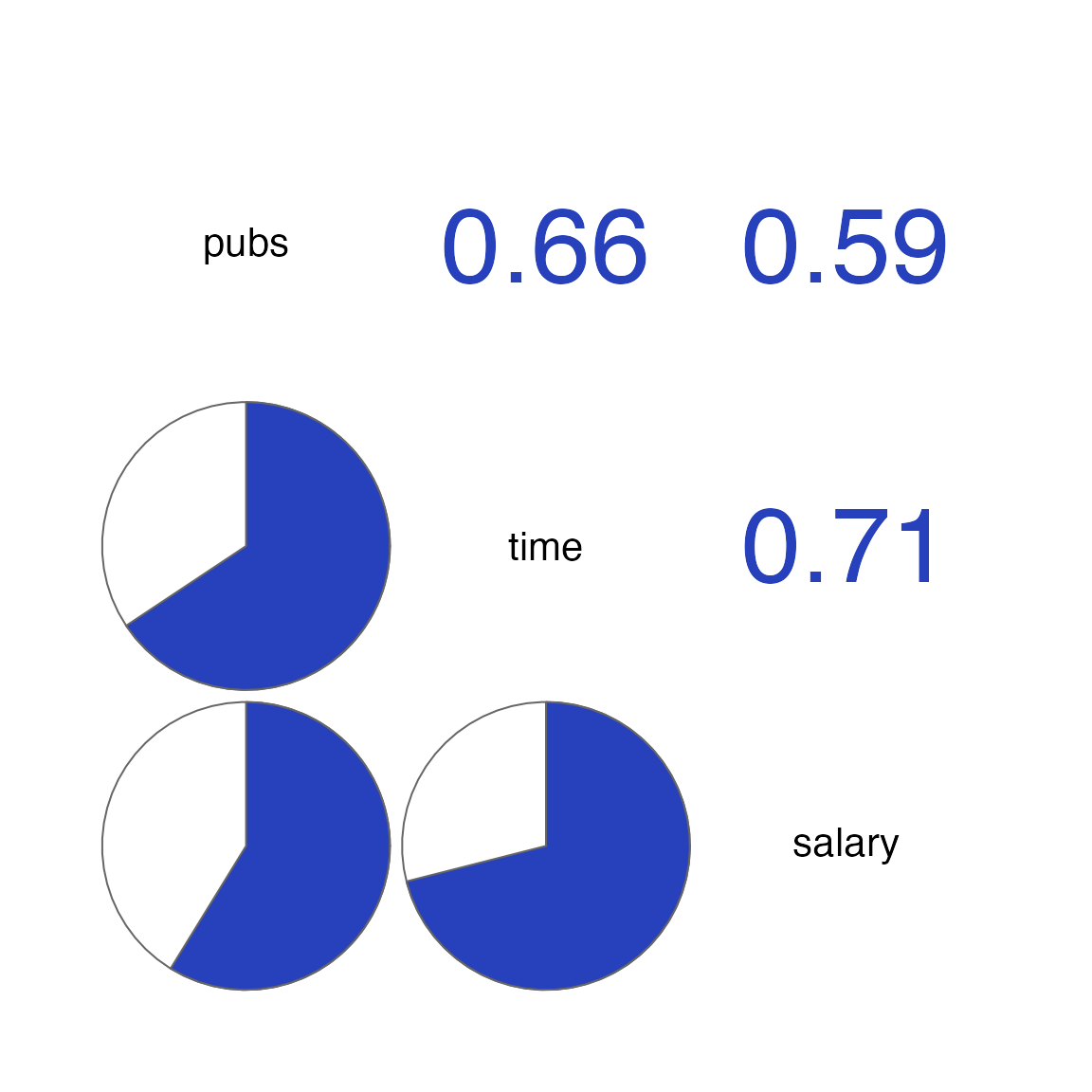
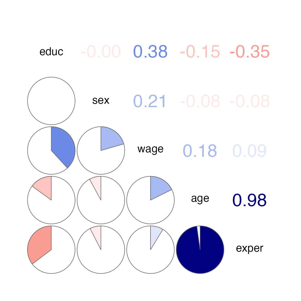
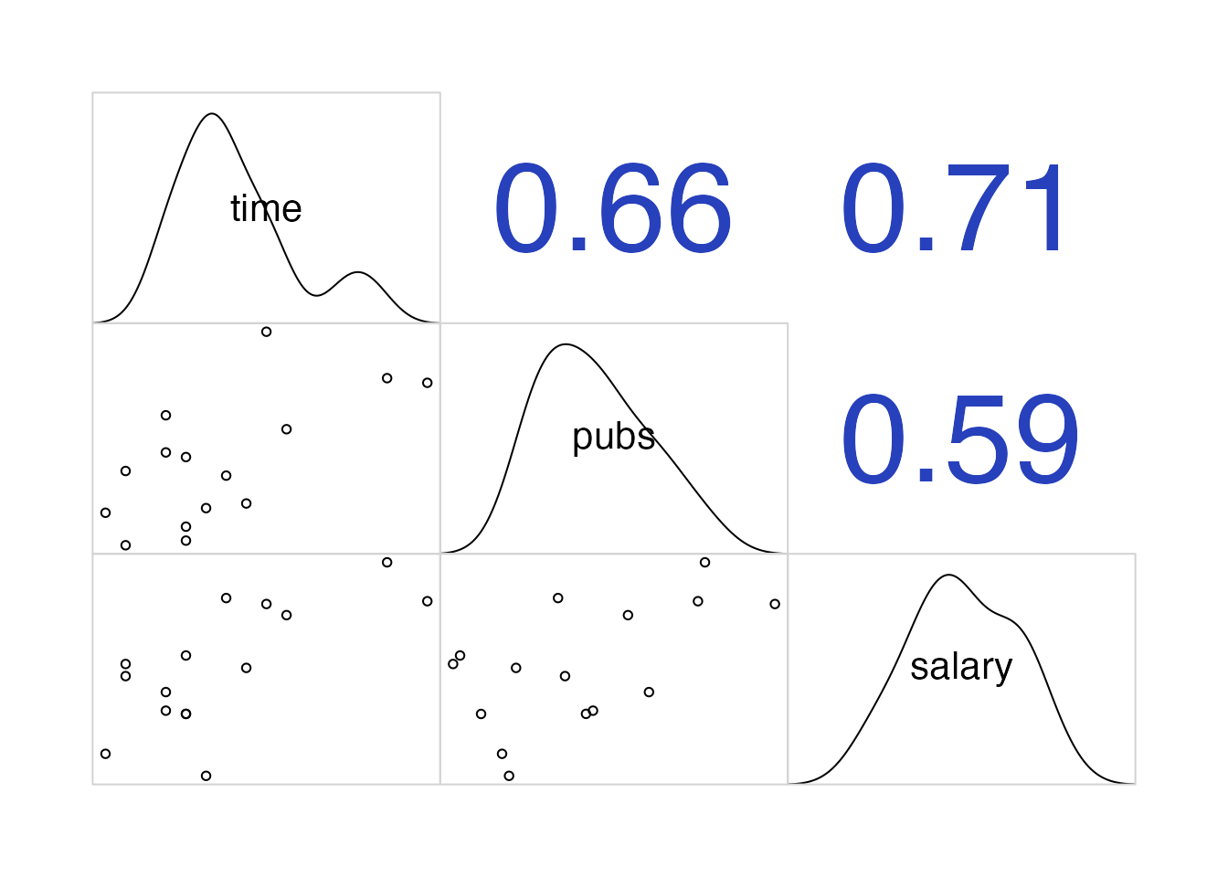
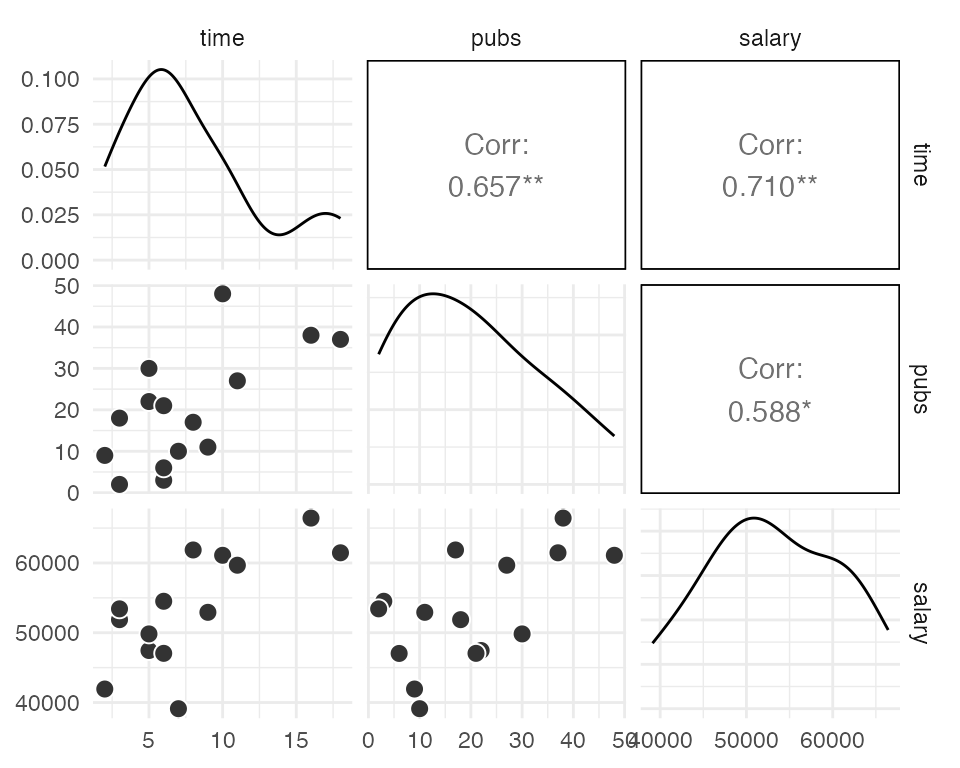
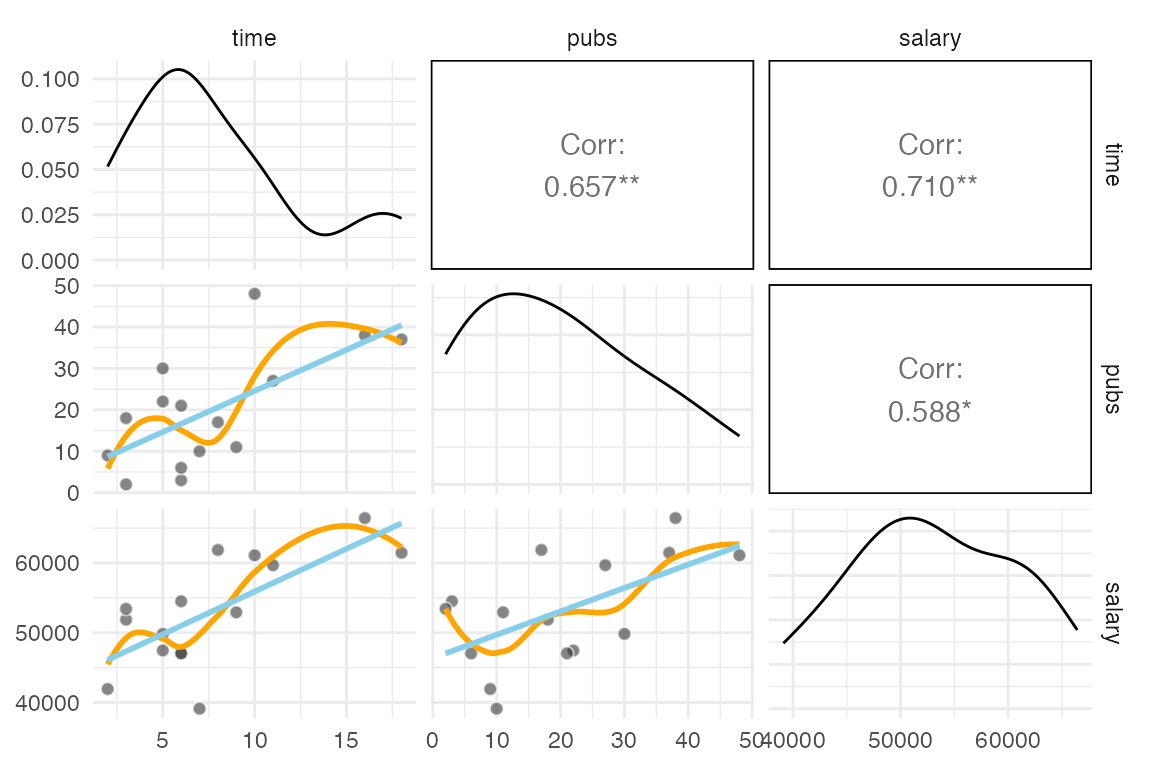
library(corrgram)corrgram(acad0,order =TRUE, # 상관계수가 높은 변수들을 가까이 위치시킴upper.panel = panel.cor, # 상관계수lower.panel = panel.pie, # 파이 차트)
tip: use a function
corgrm <-function(df, order =TRUE){corrgram(df,order = order, # 상관계수가 높은 변수들을 가까이 위치시킴upper.panel = panel.cor, # 상관계수lower.panel = panel.pie, # 파이 차트 )}corgrm(acad0)corgrm(acad0, order =FALSE)
Data from the 1985 Current Population Survey (CPS85)
임금, 교육수준, 연차, 나이, 성별 간의 상관관계
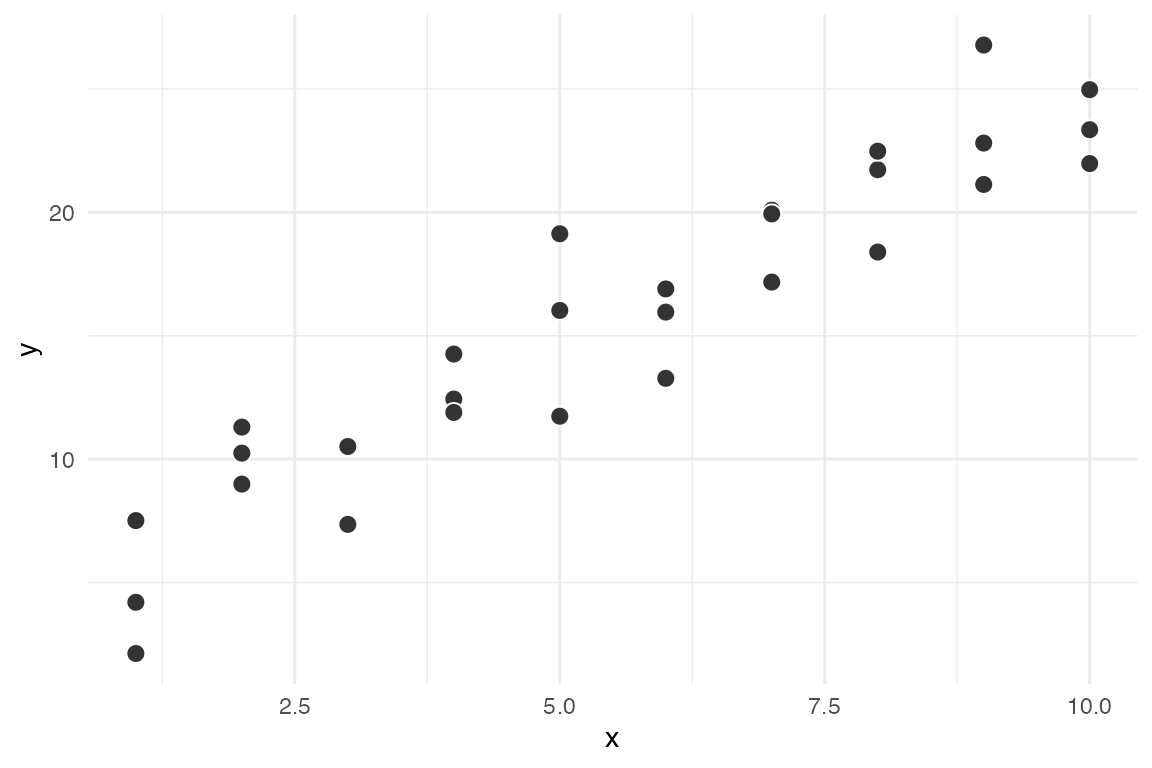
앞의 예는 \(n=1\) 에 해당하며, \(Y =a_0 +a_1X_1\)에 대해서 다음과 같이 편리하게 적용할 수 있음
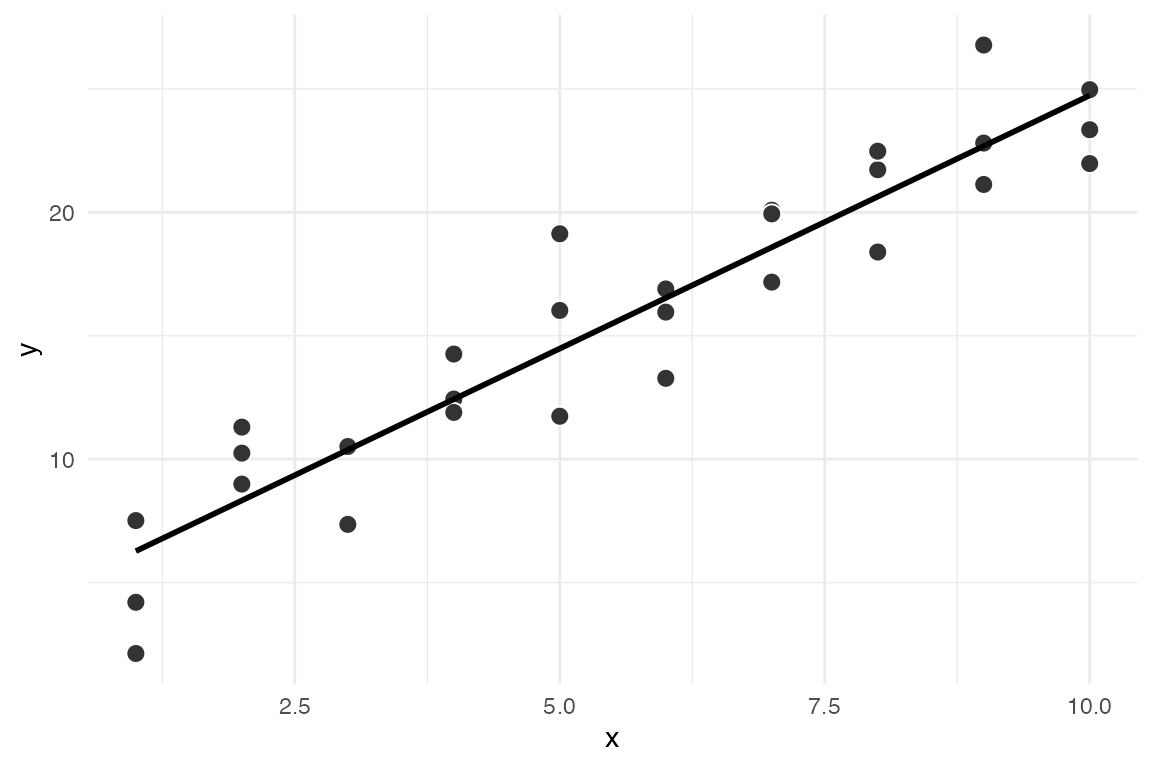
sim1_mod <-lm(y ~ x, data = sim1)coef(sim1_mod) # 모델의 parameter 즉, coefficients를 내줌#> (Intercept) x #> 4.220822 2.051533 # 위에서 구한 파라미터값과 동일함
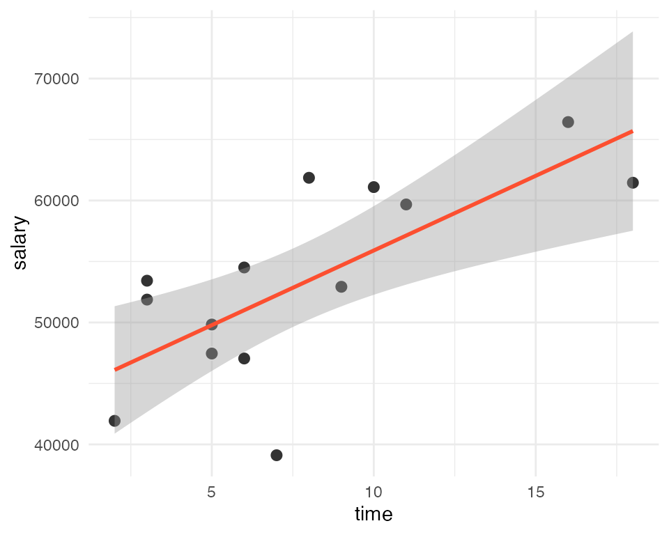
즉, 앞의 데이터에 최적인 선형 모형은 \(Y = 4.22 + 2.05X\)
lm()은 formulay ~ x를 \(Y =a_0 +a_1X\) 로 변환해 줌; Y 절편은 formula에서 생략
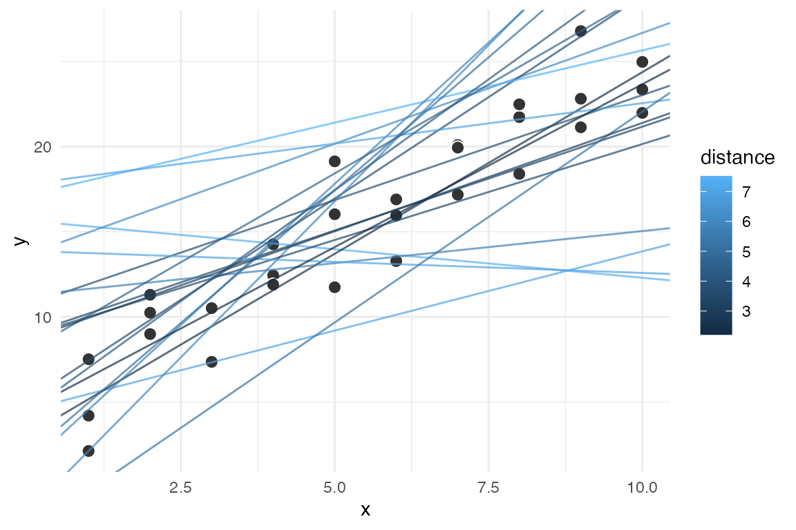
OLS estimation인 경우 알고리즘적이 아닌, 방정식의 해를 구하듯 exact form으로 최소값을 구함
\(n=2\) 인 경우인 두 변수 \(X_1\), \(X_2\)로 \(Y\)를 예측하는 경우,
lm(y ~ x1 + x2, data = df)
Note
This formula notation is called “Wilkinson-Rogers notation”, and was initially described in Symbolic Description of Factorial Models for Analysis of Variance by G. N. Wilkinson and C. E. Rogers
위에서 y ~ x라는 formula는 x, y라는 변수를 바로 evaluate하지 않고, \(Y = a_0 + a_1X\)로 해석되어 함수로 전환됨
Visualising models
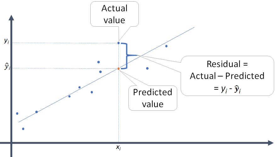
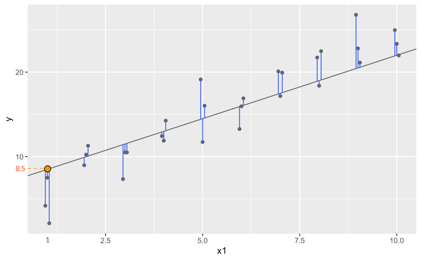
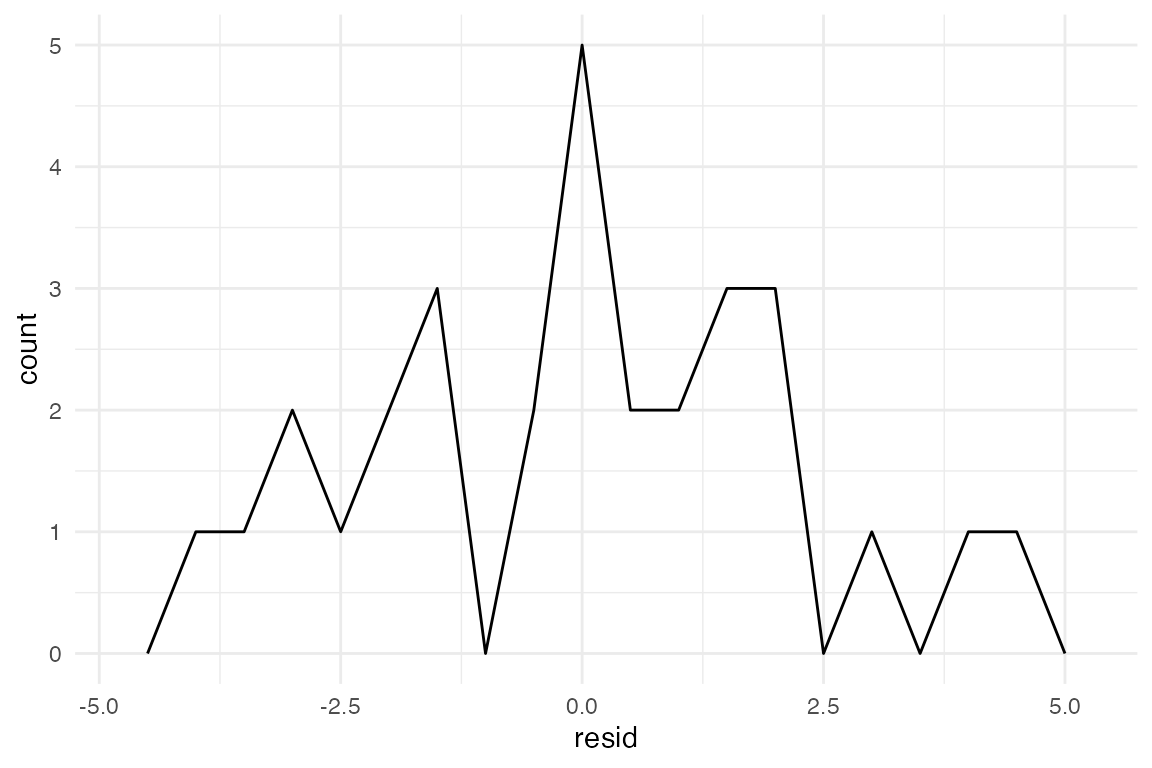
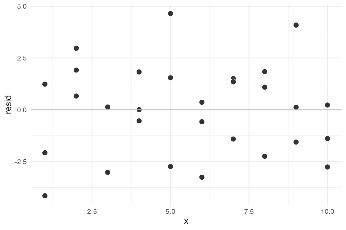
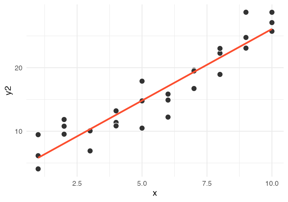
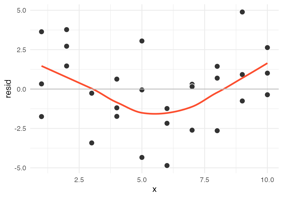
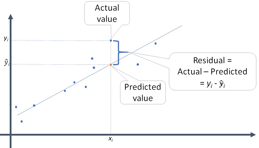
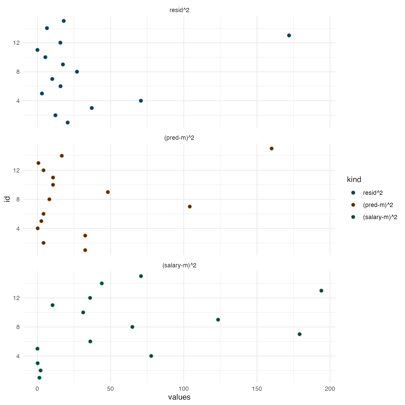
Fitted models을 이해하기 위해 모델이 예측하는 부분(prediction)과 모델이 놓친 부분(residuals)을 시각화해서 보는 것이 유용함
Predictions: the pattern that the model has captured
Residuals: what the model has missed; 통계 분석의 핵심 요소
즉, 추가된 예측 변수에 의해 설명되는 변량 정도가 sampling error, 즉 표본 추출에 따른 우연성에 의해 나타날 수 있을 확률을 계산
anova(mod1)
Analysis of Variance Table

Response: salary
          Df Sum Sq Mean Sq F value Pr(>F)
time       1 439.75  439.75  13.241  0.003 **
Residuals 13 431.73   33.21
---
Signif. codes:  0 '***' 0.001 '**' 0.01 '*' 0.05 '.' 0.1 ' ' 1
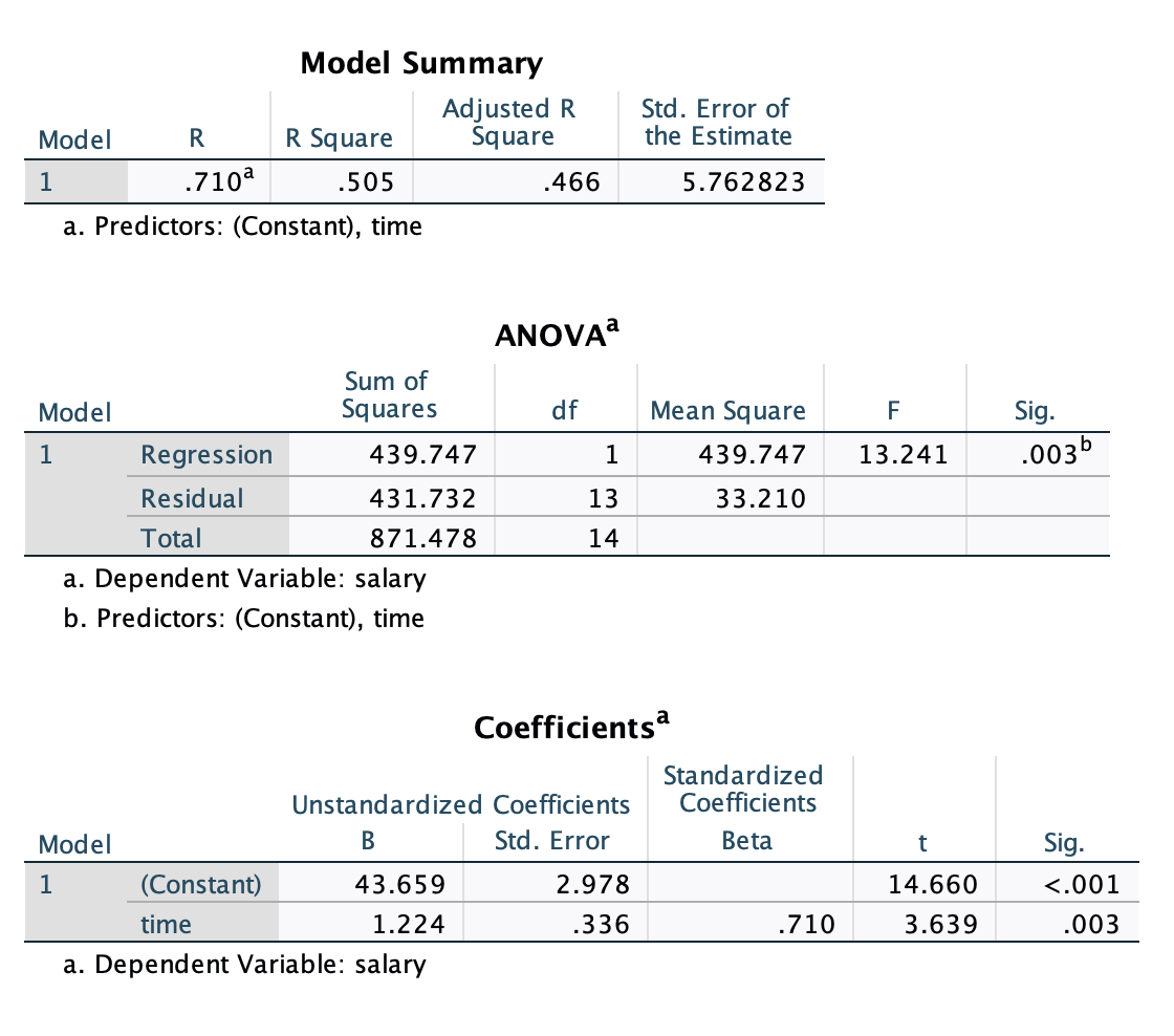
대략, (예측변수로 설명되지 않는 Y인) 잔차의 평균 변량: \(\sqrt{mean~of~SSE} = \sqrt{33.21} = 5.763\)
대략 말하면, 모형이 예측한 연봉과 실제 연봉의 차이는 평균 $5,763 정도 된다는 것을 의미함
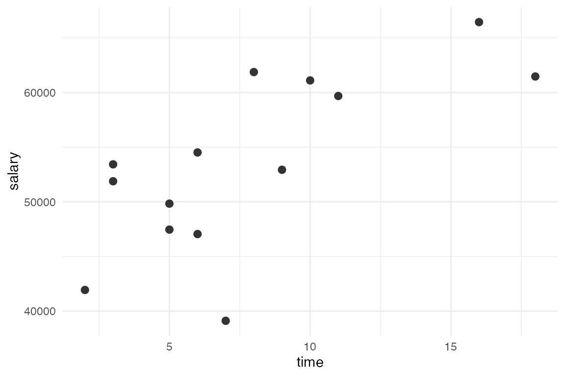
모형 \(\widehat{salary} = a_0 + a_1time\) 에 대한
SPSS 결과 테이블:
df <- acad0 |>mutate(salary = salary /1000)mod1 <-lm(salary ~ time, data = df)summary(mod1)
Call:
lm(formula = salary ~ time, data = df)

Residuals:
     Min       1Q   Median       3Q      Max
-13.1143  -3.9644   0.0514   4.0251   8.4093

Coefficients:
            Estimate Std. Error t value Pr(>|t|)
(Intercept)  43.6586     2.9780  14.660 1.83e-09 ***
time          1.2244     0.3365   3.639    0.003 **
---
Signif. codes:  0 '***' 0.001 '**' 0.01 '*' 0.05 '.' 0.1 ' ' 1

Residual standard error: 5.763 on 13 degrees of freedom
Multiple R-squared:  0.5046,    Adjusted R-squared:  0.4665
F-statistic: 13.24 on 1 and 13 DF,  p-value: 0.003
Important
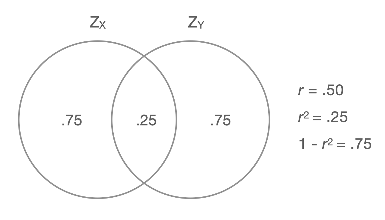
\(R^2\) 는 모형이 predictor들로부터 Y의 변량을 얼마나 예측/설명해주는지에 대한 지표로서 가장 널리 쓰임.
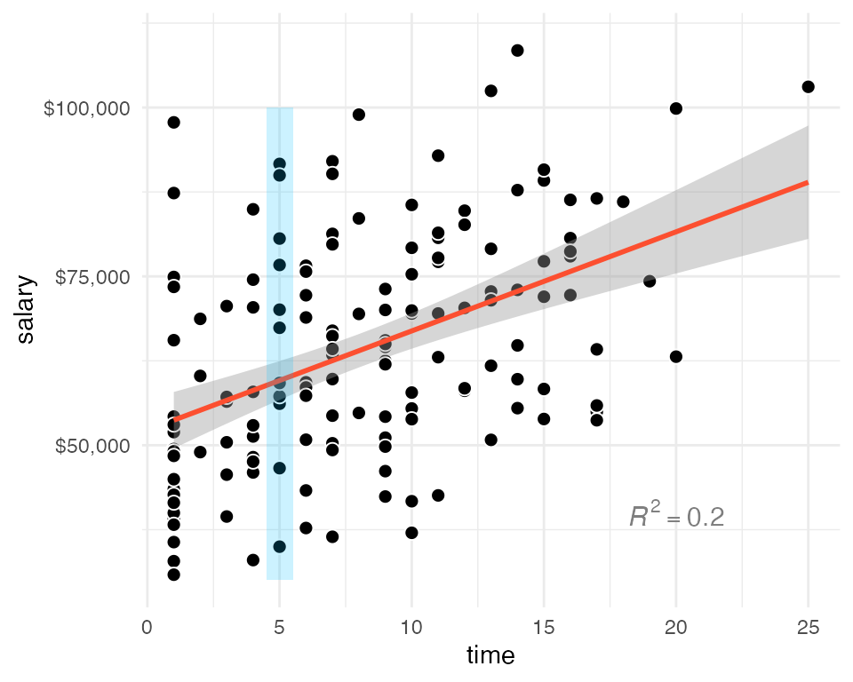
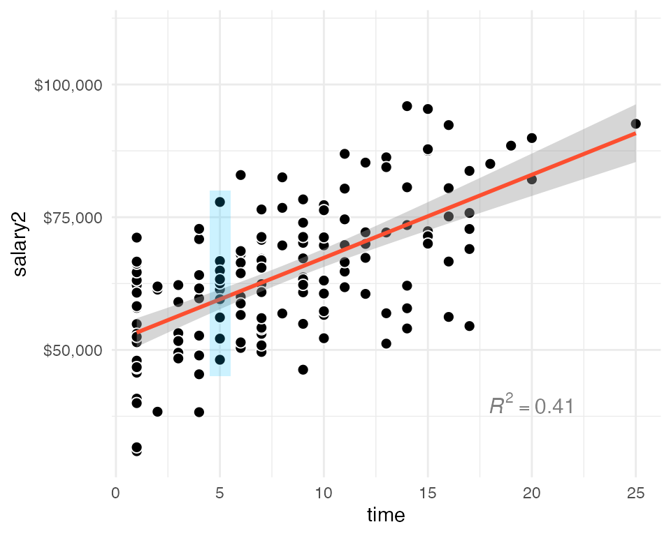
다음의 두 경우는 1년의 연차가 $1,224의 연봉 증가로 나타나는 동일한 관계를 보여주지만, 그 strength of association에는 큰 차이가 있음
Exercises
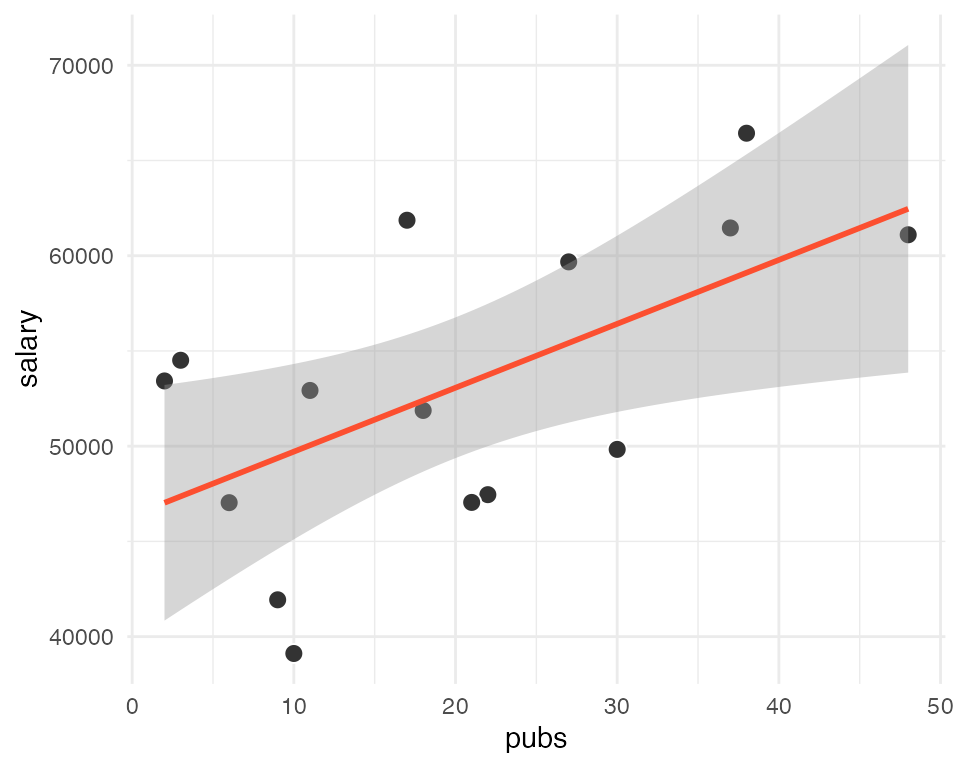
출판물의 수(pubs)가 연봉(salary)에 어떻게 영향을 미치는지 살펴보세요.
Case 2
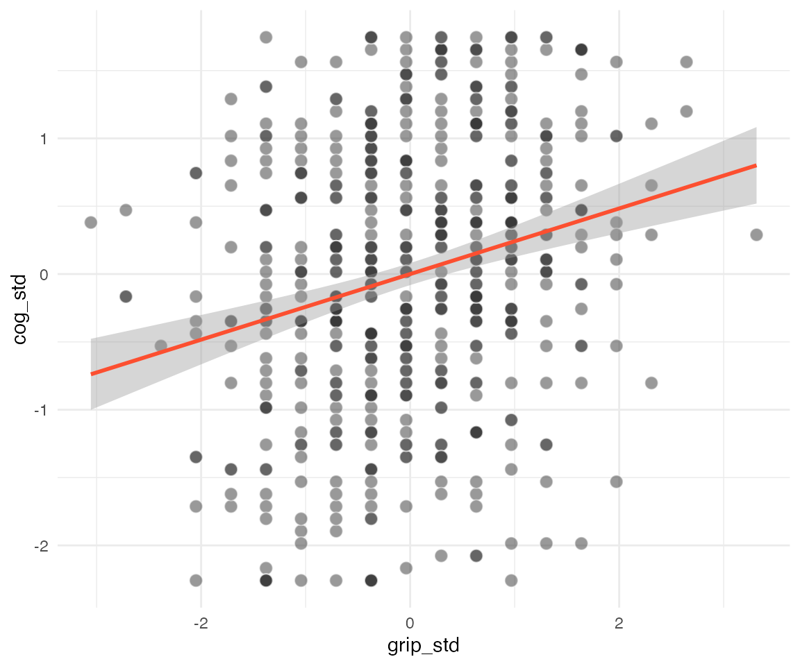
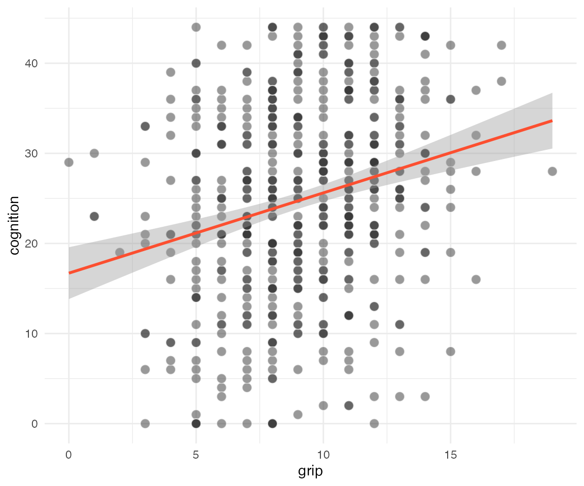
다음 데이터는 the Octogenarian Twin Study of Aging에서 나타나는 패턴을 기반으로 생성한 데이터
includes 550 older adults age 80 to 97 years.
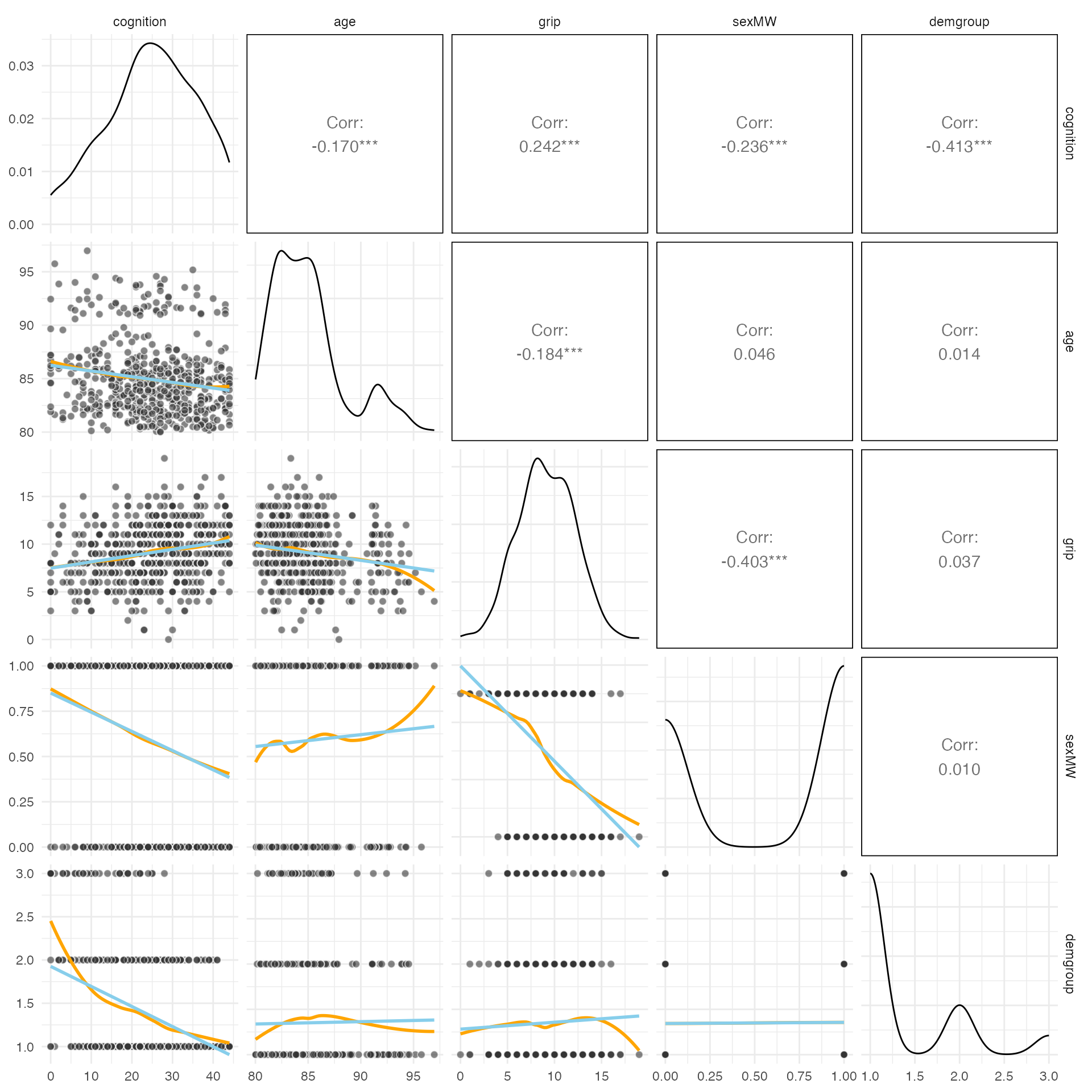
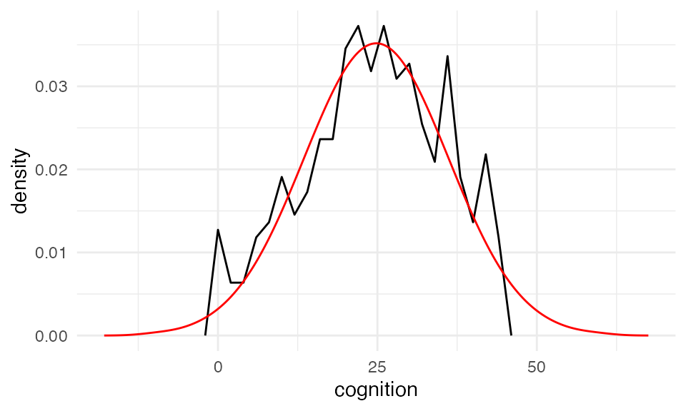
Cognition was assessed by the Information Test, a measure of general world knowledge (i.e., crystallized intelligence; range = 0 to 44)
demgroup 1: those who will not be diagnosed with dementia (none group = 1; 72.55%),
demgroup 2: those who will eventually be diagnosed with dementia later in the study (future group = 2; 19.82%)
demgroup 3: those who already have been diagnosed with dementia (current group = 3; 7.64%)
MODEL INFO:
Observations: 550
Dependent Variable: cognition
Type: OLS linear regression

MODEL FIT:
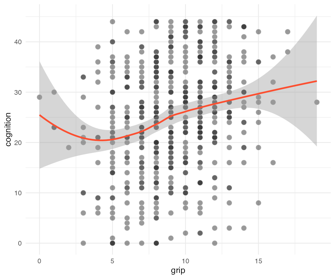
F(1,548) = 34.04, p = 0.00
R² = 0.06
Adj. R² = 0.06

Standard errors:OLS
-----------------------------------------------
                    Est.   S.E.   t val.      p
----------------- ------ ------ -------- ------
(Intercept)         0.00   0.04     0.00   1.00
grip                0.24   0.04     5.83   0.00
-----------------------------------------------

Continuous variables are mean-centered and scaled by 1 s.d.
Case 3
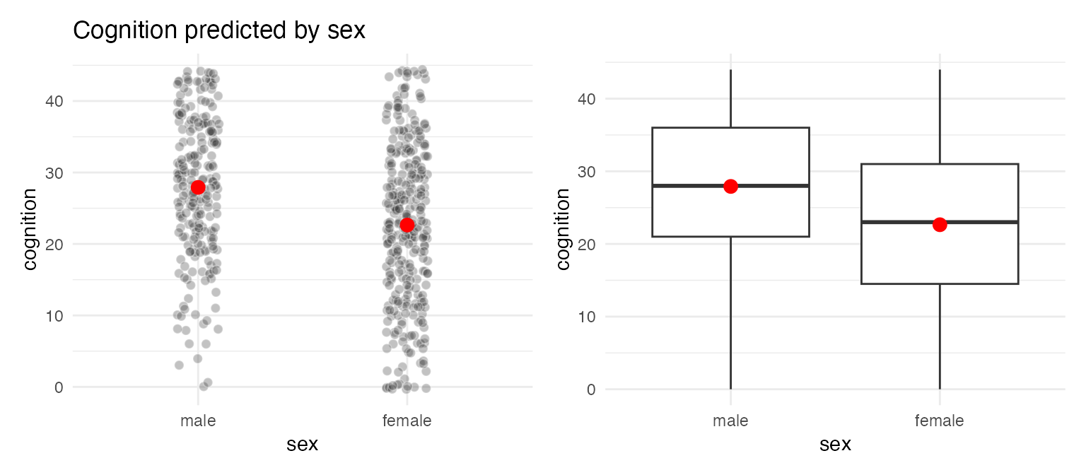
성별에 따라 인지능력(cognition)에 차이가 있는가?
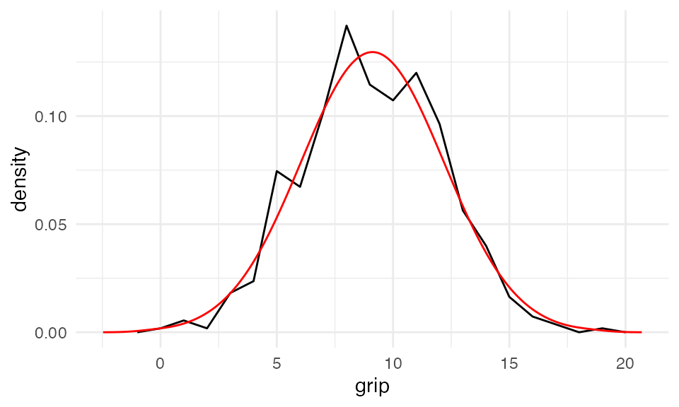
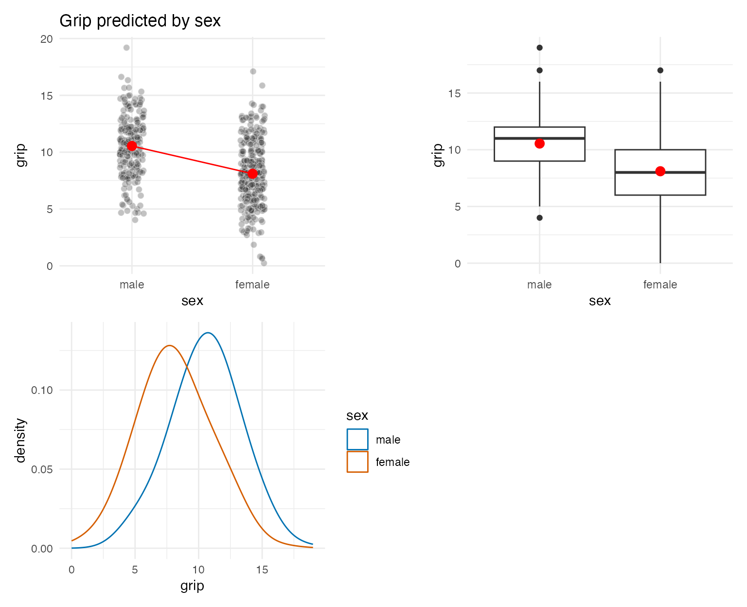
성별에 따라 악력(grip)에 차이가 있는가?
우선, 잔차의 합이 0이므로 \(\displaystyle \sum_{i=1}^{n}{(y_i - \hat{y})} = 0,~~ \hat{y} = \frac{\sum_{i=1}^{n}{y_i}}{n}\) for each \(x\)
즉, 각 카테고리 값에 대해서 모형은 평균으로 예측
기울기 -2.44는 남성과 여성의 평균 악력 차이를 의미함; 남성(0)에서 여성(1)로 1증가할 때, 악력의 증가량
절편 10.55는 남성(0)일 때의 평균 악력을 의미함.
따라서, 여성의 평균 약력은 -2.44 * (1) + 10.55 = 8.11
\(R^2\)= 0.16; 성별로 악력의 변량의 16%를 설명할 수 있음.
# A tibble: 10 × 5
    grip sex    sexfemale  pred  resid
   <dbl> <fct>      <dbl> <dbl>  <dbl>
 1     9 female         1  8.11  0.895
 2    11 male           0 10.5   0.454
 3    12 male           0 10.5   1.45
 4     6 female         1  8.11 -2.11
 5     9 female         1  8.11  0.895
 6    11 male           0 10.5   0.454
 7    10 female         1  8.11  1.89
 8     9 male           0 10.5  -1.55
 9    11 male           0 10.5   0.454
10    10 male           0 10.5  -0.546
anova(mod_grip)
Analysis of Variance Table

Response: grip
           Df Sum Sq Mean Sq F value    Pr(>F)
sex         1  794.3  794.33  106.41 < 2.2e-16 ***
Residuals 548 4090.7    7.46
---
Signif. codes:  0 '***' 0.001 '**' 0.01 '*' 0.05 '.' 0.1 ' ' 1
Dummmy coding
Formula는 factor/카테고리 변수가 predictor인 경우 카테고리 값(levels)들을 수치화해줌.
여러 방식이 있느나, 기본은 dummy coding으로, 각 카테고리를 0과 1로 표현하며, memership으로 이해하는 것이 적절함.
그 값을 새로운 변수인 dummy variable/indicator variable로 만드는데, 1에 해당하는 level을 변수명에 표시함.
예를 들어, 다음과 같이 female에 속하면(membership) 1, female에 속하지 않으면 0
Sequential coding, Helmert coding, effect coding 등등 여러 다른 coding 방식에 대해서는 책을 참고.
10.1 Alternative Coding Systems in Regression Analysis and Linear Models by Richard B. Darlington & Andrew F. Hayes
두 집단 간 차이: t-test
전통적으로 카테고리 변수에 대한 분석은 ANOVA 프레임워크에서 실시되었음.
특히, 위의 경우와 같이 두 집단 간의 차이, 즉 남성과 여성의 약력의 평균 차이를 분석할 때 t-test를 실시.
t.test(grip ~ sex, data = cognition, var.equal =TRUE) # variance가 동일하다는 가정
    Two Sample t-test

data:  grip by sex
t = 10.316, df = 548, p-value < 2.2e-16
alternative hypothesis: true difference in means between group male and group female is not equal to 0
95 percent confidence interval:
 1.976174 2.905811
sample estimates:
  mean in group male mean in group female
           10.546256             8.105263
Factor의 levels을 formula 안에서 간단히 변경하려면, fct_relevel()
mod_grip2 <-lm(grip ~fct_relevel(sex, "female"), data = cognition)# 또는 relevel(sex, ref = "female")model_matrix(cognition, mod_grip2)